Bipartite Graph Loopy Belief Propagation
In this document, we demonstrate a bipartite graph inference using loopy belief propagation. This experiment serves as a proof-of-concept for future implementation of large scale graph-based inference.
%matplotlib inline

import opengm
import matplotlib.pyplot as plt
import matplotlib.cm as cm
import numpy as np
import Image
import networkx as nx
from networkx.algorithms import bipartite
Basic Setup
- A bipartite graph \(G=(V,E)\), where the vertices are partitioned into two groups: \(V=V_0\cup V_1\), \(V_0\cap V_1=\emptyset\); the sets \(V_0\), \(V_1\) are totally disconnected.
- Each vertex stands for a Bernoulli random variable, and each edge represents a factor. Therefore, the scope of any factor contains exactly two vertices, one from each of \(V_0\) and \(V_1\).
- Initially, the marginal distribution of some of the random variables in \(V_0\) are known; all the rest of the marginal distributions are set to be uniform. The edge potentials (i.e., joint distributions determined by the factor) are set to be the tensor product of the marginal distributions of the two vertices linked by the edge.
- Marginal distributions of some of the random variables associated with the vertices in \(V_0\) are known; all other marginals are assumed uniform. All messages are initialized as \(1\).
A Toy Example
Consider the following bipartite graph
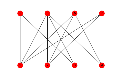
where nodes \(1\), \(2\), \(3\), \(4\) each represents a domain, while \(5\), \(6\), \(7\), \(8\) each stands for a property of the domain (e.g., certain registrant name, phone number, address, etc.). We assume the counts of infringing (denoted as \(I\)) and non-infringing (denoted as \(N\)) are known for only domains \(1\), \(2\); marginal probability distributions for nodes \(3\), \(4\) to generate infringing websites are to be inferred. Along the way, we shall also obtain the marginal probability distribution for property nodes \(5\), \(6\), \(7\), \(8\) to produce infringing websites.
The \(I\) vs. \(N\) counts for nodes \(1,2\) are listed in the following table.
| Node | \(I\) | \(N\) |
|---|---|---|
| \(1\) | 85 | 15 |
| \(2\) | 52 | 48 |
In this toy example, node \(1\) is connected to \(5,6,7,8\), while node \(2\) is only connected to \(5,6,7\). Note that node \(1\) is much more likely to generate infringing websites compared to node \(2\); it is reasonable to conjecture that this biase results from the connectivity between node \(1\) and node \(8\). Among the nodes whose marginal probability distributions are to be inferred, node \(3\) connects to node \(8\) but node \(4\) doesn't. We thus expect a higher probability of generating infringing websites for node \(3\) than node \(4\). In fact, since \(4\) connects to exactly the same properties as node \(2\), we expect the marginal prbability distributions of node \(4\) to be close to those of node \(2\).
We assume each node \(j\) is assigned a Bernoulli random variable \(X_j\) (\(1\leq j\leq 8\)). The potential functions on each node represents the prior belief for the corresponding random variable, estimated from the data if possible:
Potential functions at each property node:
On each edge we need to specify the conditional probability of a domain node producing an infringing website given the state of the propety node. We assume there is a constant probability \(\beta\in\left[0,1\right]\) for the domain node to behave the same way as the property node, e.g.,
Let us construct the graph in OpenGM. Click here for a user/developer manual.
numVar = 8
numLabels = 2
beta = 0.75
numberOfStates = np.ones(numVar, dtype=opengm.index_type)*numLabels
gm = opengm.graphicalModel(numberOfStates, operator="multiplier")

Edges = np.array([(1,5), (1,6), (1,7), (1,8), (1,6), (2,5), (2,6), (2,7), (3,8), (3,5), (3,6), (4,5), (4,6), (4,7)])
DomainNodes = set(Edges[:,0])
PropertyNodes = set(Edges[:,1])

DomainNodeCounts = np.array([[85,15],[52,48],[0,0],[0,0]])
# DomainNodeCounts = np.array([[99,1],[0,100],[0,0],[0,0]])
PropertyNodeCounts = []
for p in xrange(len(PropertyNodes)):
    PropertyNodeCounts.append([0.0, 0.0])
    for v in Edges[Edges[:,1] == (p+1+len(DomainNodes)),:][:,0]:
        PropertyNodeCounts[p] += DomainNodeCounts[v-1]

unaries = np.vstack([DomainNodeCounts, np.array(PropertyNodeCounts)])

for x in xrange(unaries.shape[0]):
    if (sum(unaries[x]) == 0.0) :
        unaries[x] = np.array(np.ones(numLabels) / sum(np.ones(numLabels)))
    else:
        unaries[x] = np.array(unaries[x] / sum(unaries[x]))

for r in xrange(unaries.shape[0]):
    fid = gm.addFunction(unaries[r])
    gm.addFactor(fid, r)

for c in xrange(Edges.shape[0]):
    fid = gm.addFunction(np.array([[beta, 1-beta], [1-beta, beta]]))
    gm.addFactor(fid, np.array(Edges[c]-1, dtype=opengm.index_type))
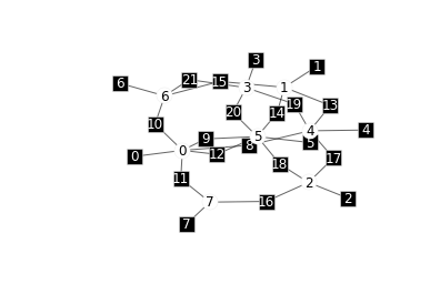
Visualize the factor graph corresponding to the graphical model. Note that in the graphical model the node subindex starts with \(0\).
opengm.visualizeGm(gm,show=False,layout="neato",plotUnaries=True,
                    iterations=1000,plotFunctions=False,
                    plotNonShared=False,relNodeSize=1.0)

get node position...
....done
inferBipartite = opengm.inference.BeliefPropagation(gm,parameter=opengm.InfParam(damping=0.01,steps=100),
                                                    accumulator="integrator")
inferBipartite.infer()

print "Marginal Probabilities for Domain Nodes:"
print "++++++++++++++++++++++++++++++++++++++++++++++++++++++++++++++++++++"
for d in xrange(4):
    print "Node {0} generates infringing websites with probability {1}".format(d+1, inferBipartite.marginals(d)[0][0])
print "++++++++++++++++++++++++++++++++++++++++++++++++++++++++++++++++++++"
print ""
print "Marginal Probabilities for Property Nodes:"
print "++++++++++++++++++++++++++++++++++++++++++++++++++++++++++++++++++++"
for d in xrange(4):
    print "Node {0} generates infringing websites with probability {1}".format(d+5, inferBipartite.marginals(d+4)[0][0])
print "++++++++++++++++++++++++++++++++++++++++++++++++++++++++++++++++++++"

Marginal Probabilities for Domain Nodes:
++++++++++++++++++++++++++++++++++++++++++++++++++++++++++++++++++++
Node 1 generates infringing websites with probability 0.921084363355
Node 2 generates infringing websites with probability 0.612357558773
Node 3 generates infringing websites with probability 0.621324912368
Node 4 generates infringing websites with probability 0.593463184578
++++++++++++++++++++++++++++++++++++++++++++++++++++++++++++++++++++

Marginal Probabilities for Property Nodes:
++++++++++++++++++++++++++++++++++++++++++++++++++++++++++++++++++++
Node 5 generates infringing websites with probability 0.742725289156
Node 6 generates infringing websites with probability 0.826792875427
Node 7 generates infringing websites with probability 0.740086302281
Node 8 generates infringing websites with probability 0.878739154843
++++++++++++++++++++++++++++++++++++++++++++++++++++++++++++++++++++
As we expected, the model predicts higher infringing probability for Node \(3\) than Node \(4\); Node \(8\) has the highest probability of generating infringing websites among all property nodes.
Appendix: Loopy Belief Propagation (LBP)
1. Constructing the Cluster Graph
The first step in LBP is to construct a cluster graph from the orignal graph. This derived graph is undirected, with each node representing a cluster \(C_j\subset V\). Let us denote the number of random varaibles in \(C_j\) as \(\left|C_j\right|\). When \(C_j\cap C_k\neq \emptyset\), define a sepset \(S_{jk}\subset C_j\cap C_k\). Obviously, \(S_{jk}=S_{kj}\).
Each factor \(\phi_k\) is assigned to a unique cluster \(C_{\alpha\left(k\right)}\) in the cluster graph. This assignment should at least ensure that \(\mathrm{Scope}\left[\phi_k\right]\subset C_{\alpha\left(k\right)}\). We then construct potentials for each cluster by
Some clusters may have more than one factors assigned to them, while other clusters may have none. In the latter case, initialize the corresponding potential to be \(1\) (one can assign a uniform distribution as well, but for potentials this doesn't matter --- the results will be renormalized to get a probability distribution).
Cluster graphs are generally non-unique.
2. Message Passing
The message passed from cluster \(C_i\) to \(C_j\) is
For each pair of subscripts \((i,j)\), this formula translates into \(2^{\left|S_{ij}\right|}\) equalities. The summation involves \(2^{\left|C_i\backslash S_{ij}\right|}\) terms while the product combines \(2^{\left|N_i\right|-1}\).
This process is repeated until two messages (one for each direction) are computed for each edge.
3. Summarize Beliefs
Compute
Note that this is a total number of \(2^{\left|C_i\right|}\) equalities.