Review Notes: Curves

Lines in $\mathbb{R}^3$

A line in $\mathbb{R}^3$ can be uniquely determined by a point $P_0=\left(x_0, y_0, z_0\right)$ and a direction $\vec{v} = \left(v_x, v_y, v_z\right)$, as

$$\ell:\left\{\overrightarrow{OP_0}+t\,\vec{v}\mid t\in\mathbb{R}\right\}.$$

Equivalently, any point $P=\left(x,y,z\right)$ on $\ell$ must satisfy the parametric equation

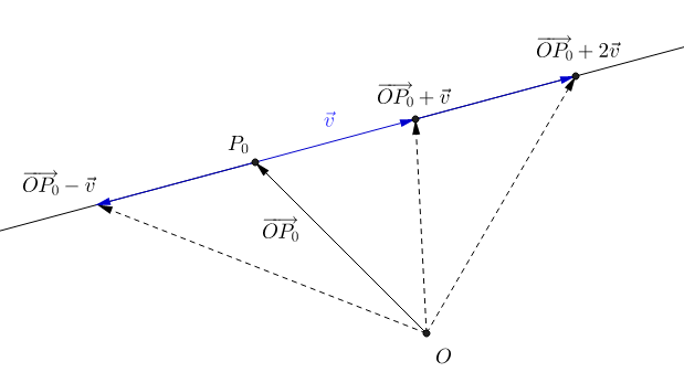
\begin{equation}\label{eq:parametricLine} \left\{ \begin{array}{rl} x &= x_0+t\,v_x,\\ y &= y_0+t\,v_y,\\ z &= z_0+t\,v_z. \end{array} \right. \end{equation}

Parametric Line

Figure 1. the parametric equation of a line

If $v_x\neq 0, v_y\neq 0, v_z\neq 0$, we can also put \eqref{eq:parametricLine} into the following symmetric equations:

\begin{equation}\label{eq:symmetricEquation} \frac{x-x_0}{v_x}=\frac{y-y_0}{v_y}=\frac{z-z_0}{v_z}. \end{equation}

Alternatively, a line in $\mathbb{R}^3$ can also be determined by two distinct points $P_0=\left(x_0, y_0, z_0\right)$, $P_1=\left(x_1, y_1, z_1\right)$. In this case, set the direction vector $\vec{v}$ in \eqref{eq:parametricLine} as

$$\vec{v}=\overrightarrow{P_0P_1}=\overrightarrow{OP_1}-\overrightarrow{OP_0}=\left(x_1-x_0, y_1-y_0, z_1-z_0\right),$$

thus any point $P=\left(x,y,z\right)$ on $\ell$ must satisfy

\begin{equation} \left\{ \begin{array}{rl} x &= x_0+t\left(x_1-x_0\right),\\ y &= y_0+t\left(y_1-y_0\right),\\ z &= z_0+t\left(z_1-z_0\right). \end{array} \right. \end{equation}

Parametric Curves in $\mathbb{R}^3$

In the parametric equation \eqref{eq:parametricLine}, coordiantes $x,y,z$ are functions of $t$. We can denote the tuple $\left(x,y,z\right)$ as a vector-valued function of $t$:

$$\vec{r}\left(t\right)=\left(x_0+t\,v_x,y_0+t\,v_y,z_0+t\,v_z\right)=:\left(x\left(t\right),y\left(t\right),z\left(t\right)\right).$$

Taking one step further, $x\left(t\right), y\left(t\right), z\left(t\right)$ can be much more general functions than linear ones. Each vector-valued funciton of a single variable gives rise to a parametric curve

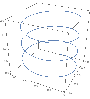
\begin{equation}\label{eq:parametricCurve} \vec{r}\left(t\right)=\left(x\left(t\right),y\left(t\right),z\left(t\right)\right). \end{equation}

Helix

Example. Let

$$x\left(t\right)=\cos 10t,\quad y\left(t\right)=\sin 10t,\quad z\left(t\right)=t$$

where $t\in\left(-\infty,\infty\right)$. Then

$$\vec{r}\left(t\right)=\left(\cos 10t, \sin 10t, t\right)$$

is a helix in $\mathbb{R}^3$ (see the figure on the right).

Remark. It is worth noting that the parametrizations of curves are not unique. For instance, the helix in the example above can be equivalently parametrized as

$$\vec{r}\left(t\right)=\left(\cos t,\sin t, \frac{t}{10}\right)$$

where $t\in\left(-\infty,\infty\right)$. One way to understand this is to consider parametrization as a physical motion, where $t$ stands for time and $\vec{r}\left(t\right)$ is the location of a point mass. The curve is the trace of $\vec{r}\left(t\right)$ in time, but the same trace can be generated from an infinite number of possible motions. For instance, the point mass may move with constant speed, or go back and forth, or stop moving every five minutes......

Example. The following two sets of parametrization equations

\begin{align*} \ell_1:\quad &\vec{r}_1\left(t\right) = \left(1,0,0\right)+t\left(1,2,1\right),\\ \ell_2:\quad &\vec{r}_2\left(t\right) = \left(2,2,1\right)+t\left(2,4,2\right). \end{align*}

To see this, notice that $\ell_1$ is parallel to the vector $\left(1,2,1\right)$ and $\ell_2$ is parallel to the vector $\left(2,4,2\right)=2\cdot\left(1,2,1\right)$, which means that $\ell_1,\ell_2$ are parallel to each other. Moreover, notice that point $\left(2,2,1\right)$ lies on both $\ell_1$ and $\ell_2$

\begin{align*} \ell_1\left(1\right) &= \left(1,0,0\right)+\left(1,2,1\right)=\left(2,2,1\right),\\ \ell_2\left(0\right) &= \left(2,2,1\right)+\left(0,0,0\right)=\left(2,2,1\right), \end{align*}

thus $\ell_1,\ell_2$ are the same line.

All standard differential and integral operations can be defined on vector-valued functions; one just need to apply the operations to each component. Assume $\vec{r}\left(t\right)=\left(x\left(t\right),y\left(t\right),z\left(t\right)\right)$, then the derivative of $\vec{r}\left(t\right)$ is

$$\frac{d}{dt}\vec{r}\left(t\right)=\left(\frac{d}{dt}x\left(t\right),\frac{d}{dt}y\left(t\right),\frac{d}{dt}z\left(t\right)\right).$$

When the context is clear, one can also write the derivative of $\vec{r}\left(t\right)$ with the prime notation:

$$\vec{r}'\left(t\right)=\left(x'\left(t\right),y'\left(t\right),z'\left(t\right)\right).$$

Major rules of derivatives from single-variable calculus still holds for vector-values functions; it often suffices to replace scalar products with dot or cross products. In particular,

\begin{align*} &\left(\vec{u}\left(t\right)+\vec{u}\left(t\right)\right)'=\vec{u}'\left(t\right)+\vec{v}'\left(t\right),\\ &\left(c\vec{u}\left(t\right)\right)'=c\vec{u}'\left(t\right),\\ &\left(c\left(t\right)\vec{u}\left(t\right)\right)'=c'\left(t\right)\vec{u}\left(t\right)+c\left(t\right)\vec{u}'\left(t\right),\\ &\left(\vec{u}\left(t\right)\cdot \vec{v}\left(t\right)\right)'=\vec{u}'\left(t\right)\cdot\vec{v}\left(t\right)+\vec{u}\left(t\right)\cdot\vec{v}'\left(t\right),\\ &\left(\vec{u}\left(t\right)\times \vec{v}\left(t\right)\right)'=\vec{u}'\left(t\right)\times\vec{v}\left(t\right)+\vec{u}\left(t\right)\times\vec{v}'\left(t\right). \end{align*}

Example.

\begin{align*} \left(\vec{u}\left(t\right)\cdot\left(\vec{v}\left(t\right)\times\vec{w}\left(t\right)\right)\right)'&=\vec{u}'\left(t\right)\cdot\left(\vec{v}\left(t\right)\times\vec{w}\left(t\right)\right)+\vec{u}\left(t\right)\cdot\left(\vec{v}\left(t\right)\times\vec{w}\left(t\right)\right)'\\ &=\vec{u}'\left(t\right)\cdot\left(\vec{v}\left(t\right)\times\vec{w}\left(t\right)\right)+\vec{u}\left(t\right)\cdot\left(\vec{v}'\left(t\right)\times\vec{w}\left(t\right)+\vec{v}\left(t\right)\times\vec{w}'\left(t\right)\right)\\ &=\vec{u}'\left(t\right)\cdot\left(\vec{v}\left(t\right)\times\vec{w}\left(t\right)\right)+\vec{u}\left(t\right)\cdot\left(\vec{v}'\left(t\right)\times\vec{w}\left(t\right)\right)+\vec{u}\left(t\right)\cdot\left(\vec{v}\left(t\right)\times\vec{w}'\left(t\right)\right). \end{align*}

Similar to the derivative, the integral and anti-derivative of $\vec{r}\left(t\right)$ are also defined component-wise:

\begin{align*} \int_a^b\vec{r}\left(t\right)dt&=\left(\int_a^bx\left(t\right)dt,\int_a^by\left(t\right)dt,\int_a^bz\left(t\right)dt\right),\quad\textrm{(integral)}\\ \int\vec{r}\left(t\right)dt&=\left(\int x\left(t\right)dt,\int y\left(t\right)dt,\int z\left(t\right)dt\right).\quad\textrm{(anti-derivative)} \end{align*}

Recall the difference between integral and anti-derivative in one-variable calculus. If $X\left(t\right),Y\left(t\right),Z\left(t\right)$ are real-valued functions satisfying

$$X'\left(t\right)=x\left(t\right),\quad Y'\left(t\right)=y\left(t\right),\quad Z'\left(t\right)=z\left(t\right)$$

then

\begin{align*} \int\vec{r}\left(t\right)dt&=\left(\int x\left(t\right)dt,\int y\left(t\right)dt,\int z\left(t\right)dt\right)\\ &=\left(X\left(t\right)+C_1, Y\left(t\right)+C_2, Z\left(t\right)+C_3\right)\\ &=\left(X\left(t\right), Y\left(t\right), Z\left(t\right)\right)+\left(C_1, C_2, C_3\right) \end{align*}

where $C_1, C_2, C_3$ are arbitrary constants. Moreover, it is important that the Fundamental Theorem of Calculus (FTC) holds for vector-valued functions:

\begin{align*} \int_a^b\vec{r}\left(t\right)dt&=\left(X\left(b\right)-X\left(a\right), Y\left(b\right)-Y\left(a\right), Z\left(b\right)-Z\left(a\right)\right)\\ &=\left(X\left(b\right),Y\left(b\right),Z\left(b\right)\right)-\left(X\left(a\right),Y\left(a\right),Z\left(a\right)\right). \end{align*}

Example. Write $\vec{r}'\left(t\right)=v\left(t\right)$, $\vec{v}'\left(t\right)=\vec{a}\left(t\right)$. Suppose

$$\vec{a}\left(t\right)=\left(\cos t,\sin t\right),\quad \vec{v}\left(0\right)=\left(1,2\right), \quad\vec{r}\left(0\right)=\left(3,4\right),$$

let's compute $\vec{r}\left(t\right)$. First, note that

$$\vec{v}\left(t\right)=\int\vec{a}\left(t\right)dt=\left(\int\cos t\, dt, \int\sin t\, dt\right)=\left(\sin t,-\cos t\right)+\left(C_1,C_2\right)$$

and

$$\left(1,2\right)=\vec{v}\left(0\right)=\left(0,-1\right)+\left(C_1,C_2\right)$$

thus

$$\left(C_1,C_2\right)=\left(1,2\right)-\left(0,-1\right)=\left(1,3\right)$$

from which one has

$$\vec{v}\left(t\right)=\left(\sin t,-\cos t\right)+\left(1,3\right)=\left(\sin t+1, -\cos t+3\right).$$

Next,

$$\vec{r}\left(t\right)=\int\vec{v}\left(t\right)dt=\left(\int\left(\sin t + 1\right) dt, \int\left(-\cos t + 3\right) dt\right)=\left(-\cos t + t, -\sin t +3t\right)+\left(C_3,C_4\right),$$

and we can find $C_3, C_4$ using the initial condition

$$\left(3,4\right)=\vec{v}\left(0\right)=\left(-1,0\right)+\left(C_3,C_4\right)\quad\Rightarrow\quad \left(C_3,C_4\right)=\left(4,4\right).$$

Thus

$$\vec{v}\left(t\right)=\left(4+t-\cos t, 4+3t-\sin t\right).$$

Arc-Length Parametrization

We saw from last section that the parametrization of a curve is not unique. In fact, every curve can be parametrized in inifinitely many ways: given a vector-valued function $\vec{r}\left(t\right)$, we can pick any smooth monotonic function $u\left(\tau\right)$ and compose $\vec{r}\left(t\right)$ with it, obtaining

$$\vec{r}\left(\tau\right):=\vec{r}\left(u\left(\tau\right)\right),$$

which is just a different parametrization of the same curve.

Despite the abundant choices of parametrizations available, geometry is all about properties of things that hold invariant regardless of parametrization. Arc length of a curve is one such example. Intuitively this makes sense: different parametrizations are like different ways to "draw" the curve, but arc length has nothing to do with the "drawing" process; in fact, it only depends on what is actually "drawn".

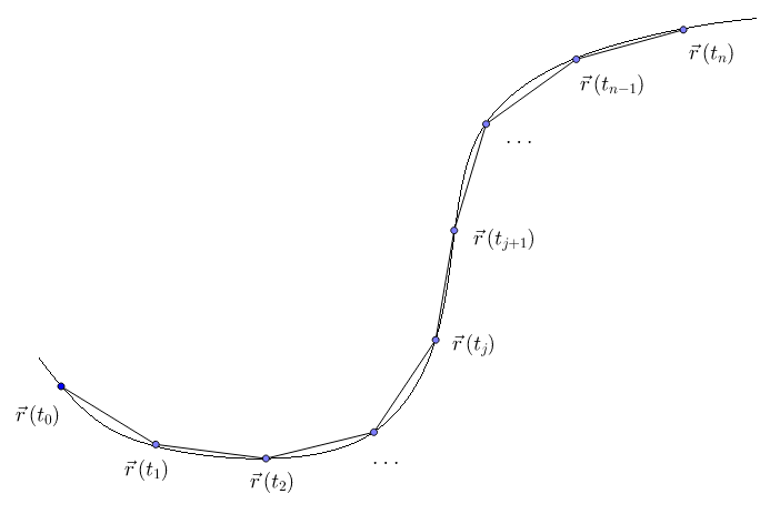
Mathematically, the arc length of a curve $\vec{v}\left(t\right)$ from time $t_0$ to time $t$ can be computed using integrals. Let

$$t_0<t_1<t_2<\cdots<t_{n-1}<t_n=:t$$

be a partition of the interval $\left[t_0, t\right]$, such that

$$\Delta t = t_{j+1}-t_j$$

is the same for all $j=0,\cdots,n-1$. When $\Delta t$ is sufficiently small, the arc length between $\vec{r}\left(t_{j}\right)$ and $\vec{r}\left(t_{j+1}\right)$ can be well approximated by the length of the line segment connecting these two points, i.e.,

\begin{align*} &\textrm{arc length between } \vec{r}\left(t_{j}\right) \textrm{ and } \vec{r}\left(t_{j+1}\right)\\ &\qquad \approx \left|\vec{r}\left(t_{j}\right) - \vec{r}\left(t_{j+1}\right)\right|. \end{align*}

Denoting $s=s\left(t\right)$ for the arc length from $\vec{r}\left(t_0\right)$ to $\vec{r}\left(t_n\right)=\vec{r}\left(t\right)$, we have

\begin{align*} s=s\left(t\right)&=\sum_{j=1}^{n-1}\textrm{arc length between } \vec{r}\left(t_{j}\right) \textrm{ and } \vec{r}\left(t_{j+1}\right)\\ &\approx \sum_{j=1}^{n-1}\left|\vec{r}\left(t_{j}\right) - \vec{r}\left(t_{j+1}\right)\right|\\ &\approx\sum_{j=1}^{n-1}\left|\vec{r}'\left(t_j\right)\Delta t\right|\\ &=\sum_{j=1}^{n-1}\left|\vec{r}'\left(t_j\right)\right|\Delta t\longrightarrow \int_{t_0}^t\left|\vec{r}'\left(\tau\right)\right|d\tau\quad\textrm{as }\Delta t\rightarrow 0. \end{align*}

Therefore, we have the following formula for the arc length computation:

\begin{equation}\label{eq:arclength} s\left(t\right)=\int_{t_0}^t\left|\vec{r}'\left(\tau\right)\right|d\tau. \end{equation}

Arc length is the very first geometric quantity among the many we are about to see in this course. Suppose $\vec{r}\left(\tau\left(\xi\right)\right)$ is another parametrization of the same curve, then the beginning and ending points of the curve should be fixed and thus

$$t_0=\tau\left(\xi_0\right),\quad t=\tau\left(\xi\right).$$

Following \eqref{eq:arclength}, the arc length under this new parametrization is

$$s\left(\xi\right)=\int_{\xi_0}^{\xi}\left|\vec{r}'\left(\xi\right)\right|d\xi.$$

However, by the chain rule

$$\vec{r}'\left(\xi\right)=\vec{r}'\left(\tau\right)\tau\left(\xi\right),$$

thus by the change-of-variables formula

\begin{align*} s\left(\xi\right)&=\int_{\xi_0}^{\xi}\left|\vec{r}'\left(\xi\right)\right|d\xi\\ &=\int_{\xi_0}^{\xi}\left|\vec{r}'\left(\tau\right)\right|\tau\left(\xi\right)d\xi\quad\textrm{(chain rule)}\\ &=\int_{t_0}^{t}\left|\vec{r}'\left(\tau\right)\right|d\tau\quad\textrm{(change of variable)}\\ &=s\left(t\right). \end{align*}

In other words, \eqref{eq:arclength} defines a quantity that is independent of the parametrization of the curve! Conventionally, we refer to such "parametrization independent" quantities as geometric quantities.

Seeing as arc length is a geometric quantity, it is canonically chosen as the "golden standard" for curve parametrization. We say that a curve is arc-parametrized if it can be written as a vector-valued function of a single variable — the arc length. The arc-length parametrization can be constructed from any parametrization* of a curve, following these steps:

Starting with an arbitrary parametrization $\vec{r}\left(t\right)$ of the curve, compute $\vec{r}'\left(t\right)$ and $\left|\vec{r}'\left(t\right)\right|$;
Compute $s=s\left(t\right)$ by \eqref{eq:arclength}, and find the inverse function $t=t\left(s\right)$;
Compose $\vec{r}\left(t\right)$ with $t=t\left(s\right)$ to obtain the arc-length parametrization of the curve $\vec{r}\left(s\right)=\vec{r}\left(t\left(s\right)\right)$.

Example. Find the arc-length parametrization of the curve

$$\vec{r}\left(t\right)=\left(\cos 3t,\sin 3t, t\right),\quad t\in\left[\frac{3\pi}{2},\frac{7\pi}{2}\right].$$

Solution. Note that

$$\vec{r}'\left(t\right)=\left(-3\sin 3t, 3\cos 3t, 1\right),\quad \left|\vec{r}'\left(t\right)\right|=\sqrt{9\sin^23t+9\cos^23t+1}=\sqrt{10}$$

thus the arc length of $\vec{r}\left(t\right)$ is

$$s = s\left(t\right)=\int_{\frac{3\pi}{2}}^t\left|\vec{r}'\left(\tau\right)\right|d\tau=\sqrt{10}\left(t-\frac{3\pi}{2}\right).$$

Inversely,

$$t = \frac{s}{\sqrt{10}}+\frac{3\pi}{2}.$$

Thus the arc-length parametrization of $\vec{r}\left(t\right)$ is

$$\vec{r}\left(s\right)=\vec{r}\left(t\left(s\right)\right)=\vec{r}\left(\frac{s}{\sqrt{10}}+\frac{3\pi}{2}\right)=\left(\cos\left(\frac{3s}{\sqrt{10}}+\frac{9\pi}{2}\right), \sin\left(\frac{3s}{\sqrt{10}}+\frac{9\pi}{2}\right), \frac{s}{\sqrt{10}}+\frac{3\pi}{2}\right).$$

A major advantage of arc-length parametrization is that it normalizes the speed of the curve.

Theorem 1. If $\vec{r}\left(s\right)$ is an arc-length parametrized curve, then $\left|\vec{r}'\left(s\right)\right|=1$.

Proof. Differentiating both sides of \eqref{eq:arclength}, we see that $s'\left(t\right)=\left|\vec{r}'\left(t\right)\right|$. Since $t=t\left(s\right)$ is the inverse function of $s=s\left(t\right)$, there holds

$$t'\left(s\right)=\frac{1}{s'\left(t\right)}=\frac{1}{\left|\vec{r}'\left(t\right)\right|}.$$

It then follows from the chain rule that

\begin{align*} \left|\vec{r}'\left(s\right)\right|=\left|\vec{v}'\left(t\right)\,t'\left(s\right)\right|=\left|\vec{v}'\left(t\right)\cdot\frac{1}{\left|\vec{v}'\left(t\right)\right|}\right|=\frac{1}{\left|\vec{v}'\left(t\right)\right|}\cdot \left|\vec{v}'\left(t\right)\right|=1. \end{align*}

$\blacksquare$

Curvature and Principal Normal Vectors

As one might infer from the name, curvature measures the "curviness" of a curve (how much it deviates from a straight line). Since the direction of tangent vectors along a line stay constant, it is natural to quantify "curviness" using the change in the direction of tangent vectors. The direction of tangent vectors is fully captured in their "unit" counterpart.

Definition. The unit tangent vector along a curve $\vec{r}\left(t\right)$ is

$$\vec{T}\left(t\right)=\frac{\vec{r}'\left(t\right)}{\left|\vec{r}'\left(t\right)\right|}.$$

Proposition 1. Under arc-length parametrization, $\vec{T}\left(s\right)=\vec{r}'\left(s\right)$.

Proof. Recall from Theorem 1 that $\left|\vec{r}'\left(s\right)\right|=1$. $\blacksquare$

We define curvature as the magnitude of the change of the unit tangent vectors under arc-length parametrization.

Definition. The curvature of a curve $\vec{r}\left(t\right)$ is

$$\kappa\left(s\right)=\left|\frac{d\vec{T}\left(s\right)}{ds}\right|.$$

There are 2 key points in this definition: (1) If one needs to compute $\kappa$ from its definition, then the curve has to be first cast into arc-length parametrization (there are also other ways to compute $\kappa$, as the textbook indicates); (2) The curvature of a curve is always non-negative (this is no longer true for the curvature of surfaces, as we shall see later in this course). According to Proposition 1, under arc-length parametrization

$$\kappa\left(s\right)=\left|\vec{r}''\left(s\right)\right|.$$

In words, for a curve under arc-length parametrization, its curvature is the magnitude of the second order derivative of the vector-valued function that represents the curve.

Example. Let us compute the curvature of the curve

$$\vec{r}\left(t\right)=\left(\cos 3t,\sin 3t, t\right),\quad t\in\left[\frac{3\pi}{2},\frac{7\pi}{2}\right].$$

Note that this is exactly the same curve for which we computed arc-length parametrization in the previous section. The arc-length parametrization is

$$\vec{r}\left(s\right)=\left(\cos\left(\frac{3s}{\sqrt{10}}+\frac{9\pi}{2}\right), \sin\left(\frac{3s}{\sqrt{10}}+\frac{9\pi}{2}\right), \frac{s}{\sqrt{10}}+\frac{3\pi}{2}\right),$$

thus

\begin{align*} \vec{r}'\left(s\right)&=\left(-\frac{3}{\sqrt{10}}\sin\left(\frac{3s}{\sqrt{10}}+\frac{9\pi}{2}\right), \frac{3}{\sqrt{10}}\cos\left(\frac{3s}{\sqrt{10}}+\frac{9\pi}{2}\right), \frac{1}{\sqrt{10}}\right),\\ \vec{r}''\left(s\right)&=\left(-\frac{9}{10}\cos\left(\frac{3s}{\sqrt{10}}+\frac{9\pi}{2}\right), -\frac{9}{10}\sin\left(\frac{3s}{\sqrt{10}}+\frac{9\pi}{2}\right), 0\right), \end{align*}

and we have

$$\kappa\left(s\right)=\left|\vec{r}''\left(s\right)\right|=\frac{9}{10}.$$

A Computational Trick. Finding the arc-length parametrization involves computing $\vec{r}'\left(t\right)$ and $\left|\vec{r}'\left(t\right)\right|$, which essentially gives $\vec{T}\left(t\right)$. But this is not good enough for curvature — we have to take the derivative of $\vec{T}\left(s\right)$, not $\vec{T}\left(t\right)$! When we move on to computing $\kappa\left(s\right)$ under the arc-length parametrization, it seems too much repeated work that we have to take derivatives of each component of $\vec{r}'\left(s\right)$ all over again. A computational trick is that one can reuse $\vec{T}\left(t\right)$ for computing $\vec{T}\left(s\right)$, as long as one recalls from chain rule

$$\vec{T}'\left(s\right)=\vec{T}'\left(t\right)\cdot t'\left(s\right).$$

Example. Find the curvature of the curve

$$\vec{r}\left(t\right)=\left(\cos t+t\,\sin t, \sin t-t\,\cos t\right),\quad t\in \left[0,\infty\right).$$

Solution. Note that

$$\vec{r}'\left(t\right)=\left(-\sin t+\sin t+t\,\cos t, \cos t-\cos t +t\,\sin t\right)=\left(t\,\cos t, t\,\sin t\right),\quad \left|\vec{r}'\left(t\right)\right|=t,$$

thus

$$\vec{T}\left(t\right)=\frac{\vec{r}'\left(t\right)}{\left|\vec{r}'\left(t\right)\right|}=\frac{1}{t}\cdot \left(t\,\cos t, t\,\sin t\right)=\left(\cos t,\sin t\right).$$

The arc length is

$$s=s\left(t\right)=\int_0^t\left|\vec{r}'\left(\tau\right)\right|d\tau=\int_0^t\tau d\tau=\frac{t^2}{2}.$$

Inversely,

$$t=t\left(s\right)=\sqrt{2s},\quad\Rightarrow\quad t'\left(s\right)=\frac{1}{\sqrt{2s}}.$$

Therefore,

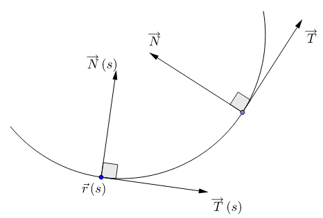
$$\kappa\left(s\right)=\left|\vec{T}'\left(s\right)\right|=\left|\vec{T}'\left(t\right)\cdot t'\left(s\right)\right|=\left|\left(-\sin t, \cos t\right)\cdot \frac{1}{\sqrt{s}}\right|=\frac{1}{\sqrt{2s}}.$$

As curvature is the magnitude of $\vec{T}'\left(s\right)$, what does the direction of $\vec{T}'\left(s\right)$ tell us? This motivates the following definition of principal normal vectors.

Definition. On a curve $\vec{r}\left(s\right)$ (arc-length parametrized) where $\kappa\left(s\right)\neq 0$, the principal normal vector is defined as

$$\vec{N}\left(s\right)=\frac{\vec{T}'\left(s\right)}{\left|\vec{T}'\left(s\right)\right|}=\frac{1}{\kappa\left(s\right)}\vec{T}'\left(s\right).$$

Remark. Note that at points $\vec{r}\left(s\right)$ where $\kappa\left(s\right)=0$ the principal normal curvature is not defined (since $\kappa\left(s\right)$ has to appear in the denominator).

Proposition. Let $s$ denote the arc-length parameter. Wherever $\vec{N}\left(s\right)$ is defined, there holds

$$\vec{N}\left(s\right)\cdot\vec{T}\left(s\right)=0.$$

Proof. Since $\left|\vec{T}\left(s\right)\right|=1$, we have

$$\vec{T}\left(s\right)\cdot\vec{T}\left(s\right)=1.$$

Differentiating both sides of the equality, we see that

$$2\vec{T}'\left(s\right)\cdot\vec{T}\left(s\right)=0.$$

Since

$$\vec{T}'\left(s\right)=\kappa\left(s\right)\vec{N}\left(s\right),$$

we conclude that

$$\kappa\left(s\right)\vec{N}\left(s\right)\cdot\vec{T}\left(s\right)=0.$$

Recall that $\kappa\left(s\right)\neq 0$ wherever $\vec{N}\left(s\right)$ is defined, thus

$$\vec{N}\left(s\right)\cdot\vec{T}\left(s\right)=0.$$

$\blacksquare$

Decompose Accerleration

For a curve $\vec{r}\left(t\right)$, $\vec{v}\left(t\right)=\vec{r}'\left(t\right)$ and $\vec{a}\left(t\right)=\vec{r}''\left(t\right)$ are often referred to as the velocity and the accerleration vector, respectively. According to the definition, the unit tangent vector $\vec{T}\left(t\right)$ is always in the same direction as $\vec{r}'\left(t\right)$. The direction of an acceleration vector is less straightforward; however, it is easy to derive that $\vec{r}''\left(t\right)$ always lives in the plane spanned by $\vec{T}$ and $\vec{N}$.

Theorem 2. The accerleration vector can be decomposed as

\begin{equation}\label{eq:accerlerationDecomposition} \vec{a}\left(t\right)=a_T\left(t\right)\vec{T}\left(t\right)+a_N\left(t\right)\vec{N}\left(t\right), \end{equation}

where

$$a_T\left(t\right)=\frac{d}{dt}\left|\vec{r}'\left(t\right)\right|,\quad a_N\left(t\right)=\kappa\left(t\right)\left|\vec{r}'\left(t\right)\right|^2.$$

Proof. Direct computation yields

\begin{align*} \vec{a}\left(t\right)&=\vec{r}''\left(t\right)=\frac{d}{dt}\left(\left|\vec{r}'\left(t\right)\right|\cdot \frac{\vec{r}'\left(t\right)}{\left|\vec{r}'\left(t\right)\right|}\right)=\frac{d}{dt}\left(\left|\vec{r}'\left(t\right)\right|\cdot\vec{T}\left(t\right)\right)\\ &=\left(\frac{d}{dt}\left|\vec{r}'\left(t\right)\right|\right)\vec{T}\left(t\right)+\left|\vec{r}'\left(t\right)\right|\frac{d}{dt}\vec{T}\left(t\right)\\ &=\left(\frac{d}{dt}\left|\vec{r}'\left(t\right)\right|\right)\vec{T}\left(t\right)+\left|\vec{r}'\left(t\right)\right|\frac{d}{ds}\vec{T}\left(s\right)s'\left(t\right)\\ &=\left(\frac{d}{dt}\left|\vec{r}'\left(t\right)\right|\right)\vec{T}\left(t\right)+\left|\vec{r}'\left(t\right)\right|\kappa\left(s\right)\vec{N}\left(s\right)\cdot\left|\vec{r}'\left(t\right)\right|\\ &=\left(\frac{d}{dt}\left|\vec{r}'\left(t\right)\right|\right)\vec{T}\left(t\right)+\kappa\left(s\right)\left|\vec{r}'\left(t\right)\right|^2\vec{N}\left(s\right). \end{align*}

The conclusion follows as we define

$$a_T\left(t\right):=\frac{d}{dt}\left|\vec{r}'\left(t\right)\right|,$$

$$a_N\left(t\right):=\kappa\left(s\right)\left|\vec{r}'\left(t\right)\right|^2=\kappa\left(s\left(t\right)\right)\left|\vec{r}'\left(t\right)\right|^2=\kappa\left(t\right)\left|\vec{r}'\left(t\right)\right|^2,$$

and conventionally write $\vec{N}\left(t\right):=\vec{N}\left(s\left(t\right)\right)=\vec{N}\left(s\right)$. $\blacksquare$

Remark. Note that $a_N\left(t\right)\geq 0$ always holds, since $\kappa\left(t\right)\geq0$ and $\left|\vec{r}'\left(t\right)\right|^2\geq 0$.

Typical questions for the decomposition of accerleration vectors involves computing $\vec{T},\vec{N},a_T,a_N,\kappa$ given curve $\vec{r}\left(t\right)$. We summarize these computations in the following "road map".

Compute $\vec{r}'\left(t\right)$ and $\vec{r}''\left(t\right)$. Both of them are straightforward derivative computations on each component of $\vec{r}\left(t\right)$.
The unit tangent vector $\vec{T}$ can be computed from its definition
$$\vec{T}\left(t\right)=\frac{\vec{r}'\left(t\right)}{\left|\vec{r}'\left(t\right)\right|}.$$
The "tangent component" of $\vec{a}\left(t\right)$, or $a_T$, can be computed from the decomposition formula \eqref{eq:accerlerationDecomposition}. In fact, dot product both sides of \eqref{eq:accerlerationDecomposition} with $\vec{T}\left(t\right)$ and using the fact that $\vec{T}\cdot\vec{N}=0$, one has
$$\vec{a}\left(t\right)\cdot\vec{T}\left(t\right)=a_T\left(t\right)\vec{T}\left(t\right)\cdot\vec{T}\left(t\right)=a_T\left(t\right),$$
or equivalently
\begin{equation}\label{eq:tangentComp} a_T\left(t\right)=\vec{r}''\left(t\right)\cdot\vec{T}\left(t\right)=\frac{\vec{r}''\left(t\right)\cdot\vec{r}'\left(t\right)}{\left|\vec{r}'\left(t\right)\right|}. \end{equation}
The "normal component" of $\vec{a}\left(t\right)$, or $a_N$, can also be computed from the decomposition formula \eqref{eq:accerlerationDecomposition}. This time we cross product both sides of \eqref{eq:accerlerationDecomposition} with $\vec{T}\left(t\right)$ and use the facts $\vec{T}\cdot\vec{N}=0$, $\vec{T}\left(t\right)\times\vec{T}\left(t\right)=0$, and
$$\left|\vec{N}\left(t\right)\times\vec{T}\left(t\right)\right|=\left|\vec{N}\left(t\right)\right|\left|\vec{T}\left(t\right)\right|\sin\left(\frac{\pi}{2}\right)=1$$
to conclude that
$$\left|\vec{a}\left(t\right)\times\vec{T}\left(t\right)\right|=\left|a_N\left(t\right)\vec{N}\left(t\right)\times\vec{T}\left(t\right)\right|=\left|a_N\left(t\right)\right|\stackrel{(*)}{=}a_N\left(t\right),$$
and thus
\begin{equation}\label{eq:normalComp} a_N\left(t\right)=\left|\vec{a}\left(t\right)\times\vec{T}\left(t\right)\right|=\frac{\left|\vec{r}''\left(t\right)\times\vec{r}'\left(t\right)\right|}{\left|\vec{r}'\left(t\right)\right|}. \end{equation}
Note that at equality $(*)$ we used the fact that $a_N\left(t\right)\geq0$ to drop the absolute value bars.
Once $a_T,a_N,\vec{T}$ are obtained, $\vec{N}$ can be very easily computed from the decomposition formula \eqref{eq:accerlerationDecomposition} as
\begin{equation}\label{eq:normalVector} \vec{N}\left(t\right)=\frac{\vec{a}\left(t\right)-a_T\left(t\right)\vec{T}\left(t\right)}{a_N\left(t\right)}=\frac{1}{a_N\left(t\right)}\left(\vec{r}''\left(t\right)-a_T\left(t\right)\frac{\vec{r}'\left(t\right)}{\left|\vec{r}'\left(t\right)\right|}\right). \end{equation}
By Theorem 2, $a_N\left(t\right)=\kappa\left(t\right)\left|\vec{r}'\left(t\right)\right|^2$, thus the curvature $\kappa$ can also be easily computed from $a_N$ as
\begin{equation}\label{eq:curvatureFromAccerleration} \kappa\left(t\right)=\frac{a_N\left(t\right)}{\left|\vec{r}'\left(t\right)\right|^2}=\frac{\left|\vec{r}''\left(t\right)\times\vec{r}'\left(t\right)\right|}{\left|\vec{r}'\left(t\right)\right|^3}. \end{equation}

Plane Curves: A Special Case

Everything we developed so far applies equally well to plane (2D) curves. The only trick is to "embed" a 2D curve into 3D by trivially attaching a $0$ at the end of the 2D vector that represents the plane curve, making the curve 3D. If one needs to find $\vec{T}$ and $\vec{N}$ for a plane curve using this trick, remember to drop the artificially attached $z$-component (thus bringing them back to 2D) at the end of the computation.

Example. Compute the curvature of the plane curve

$$t\mapsto\left(x\left(t\right),y\left(t\right)\right).$$

Solution. Let $\vec{r}\left(t\right)=\left(x\left(t\right),y\left(t\right),0\right)$. Then

\begin{align*} \vec{r}'\left(t\right)&=\left(x'\left(t\right),y'\left(t\right),0\right),\\ \left|\vec{r}'\left(t\right)\right|&=\sqrt{\left(x'\left(t\right)\right)^2+\left(y'\left(t\right)\right)^2},\\ \vec{r}''\left(t\right)&=\left(x''\left(t\right),y''\left(t\right),0\right),\\ \vec{r}''\left(t\right)\times\vec{r}'\left(t\right)&=\begin{vmatrix} \vec{i} & \vec{j} & \vec{k} \\ x'\left(t\right) & y'\left(t\right) & 0 \\ x''\left(t\right) & y''\left(t\right) & 0 \notag \end{vmatrix} =\left(x'\left(t\right)y''\left(t\right)-y'\left(t\right)x''\left(t\right)\right)\vec{k}. \end{align*}

The curvature can thus be computed from \eqref{eq:curvatureFromAccerleration} as

\begin{equation}\label{eq:curvaturePlaneCurve} \kappa\left(t\right)=\frac{\left|\vec{r}''\left(t\right)\times\vec{r}'\left(t\right)\right|}{\left|\vec{r}'\left(t\right)\right|^3}=\frac{\left|x'\left(t\right)y''\left(t\right)-y'\left(t\right)x''\left(t\right)\right|}{\left[\left(x'\left(t\right)\right)^2+\left(y'\left(t\right)\right)^2\right]^{\frac{3}{2}}}. \end{equation}

Note that this is exactly the same formula as in the textbook for plane curves (\$12.6 Equation (12)).

In principio erat Verbum

Review Notes: Curves

Lines in \(\mathbb{R}^3\)

Parametric Curves in \(\mathbb{R}^3\)

Arc-Length Parametrization

Curvature and Principal Normal Vectors

Decompose Accerleration

Plane Curves: A Special Case

Lines in \(\mathbb{R}^3\)

Parametric Curves in \(\mathbb{R}^3\)

Arc-Length Parametrization

Curvature and Principal Normal Vectors

Decompose Accerleration

Plane Curves: A Special Case

useful links

social